Supervised Dimensionality Reduction

ivis is able to make use of any provided class labels to perform supervised dimensionality reduction. Supervised ivis can thus be used in Metric Learning applications, as well as classical supervised classifier/regressor problems. Supervised embeddings can combine the distance-based characteristics of the unsupervised ivis algorithm with clear class boundaries between the class categories when trained to classify inputs simulateously to embedding them. The resulting embeddings encode relevant class-specific information into lower dimensional space, making them useful for enhancing the performance of a classifier.

ivis supports both classification and regression problems and makes use of the losses included with keras, so long as the labels are provided in the correct format.

Classification

To train ivis in supervised mode using the default softmax classification loss, simply provide the labels to the fit method’s Y parameter. These labels should be a list of 0-indexed integers with each integer corresponding to a class.

import numpy as np
from tensorflow.keras.datasets import mnist
from ivis import Ivis

(X_train, Y_train), (X_test, Y_test)  = mnist.load_data()

# Rescale to [0,1]
X_train = X_train / 255.
X_test = X_test / 255.

# Flatten images to 1D vectors
X_train = np.reshape(X_train, (len(X_train), 28 * 28))
X_test = np.reshape(X_test, (len(X_test), 28 * 28))

model = Ivis(n_epochs_without_progress=5)
model.fit(X_train, Y_train)

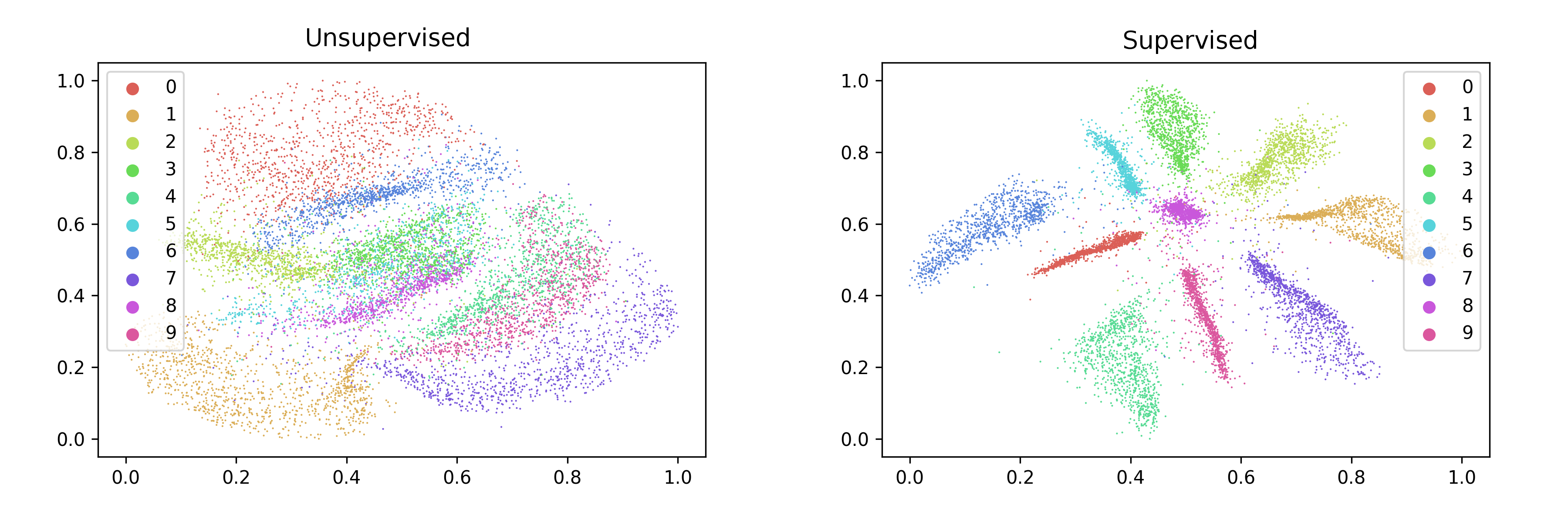
Experimental data has shown that ivis converges to a solution faster in supervised mode. Therefore, our suggestion is to lower the value of the n_epochs_without_progress parameter from the default to around 5. Here are the resulting embeddings:

Obtaining Classification Probabilities

Since training ivis in supervised mode causes the algorithm to optimize the supervised objective in conjunction with the triplet loss function, it is possible to obtain the outputs of the supervised network using the score_samples method. These may be useful for assessing the quality of the embeddings by examining the performance of the classifier, for example, or for predicting the labels for unseen data.

weight = 0.8
model = Ivis(n_epochs_without_progress=5,
             supervision_weight=weight)
model.fit(X_train, Y_train)

embeddings = model.transform(X_test)
y_pred = model.score_samples(X_test)

As before, we can train several supervised ivis models on the MNIST dataset, varying the supervision_weight parameter, coloring the plots according to the max of the returned softmax probabilities.

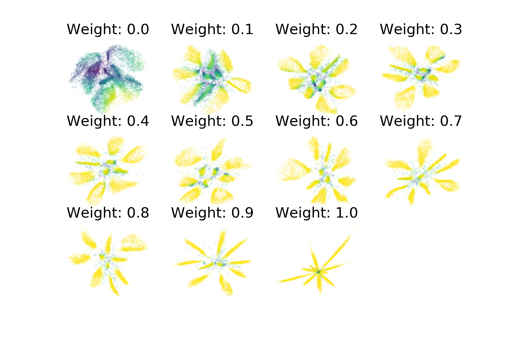
Coloring by the max softmax probabilities shows the degree of certainty in the supervised network’s predictions - areas that are yellow are predicted with a higher degree of confidence while those in blue and green have a lower degree of confidence. With low supervision weight, more of the data is classified with a low degree of certainty. Additionally, points floating in the centre between clusters tend to have lower class predictions associated with them.

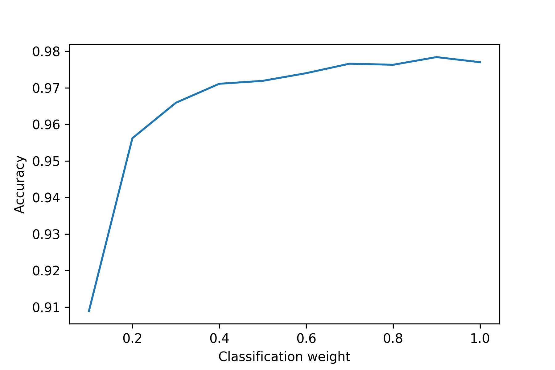
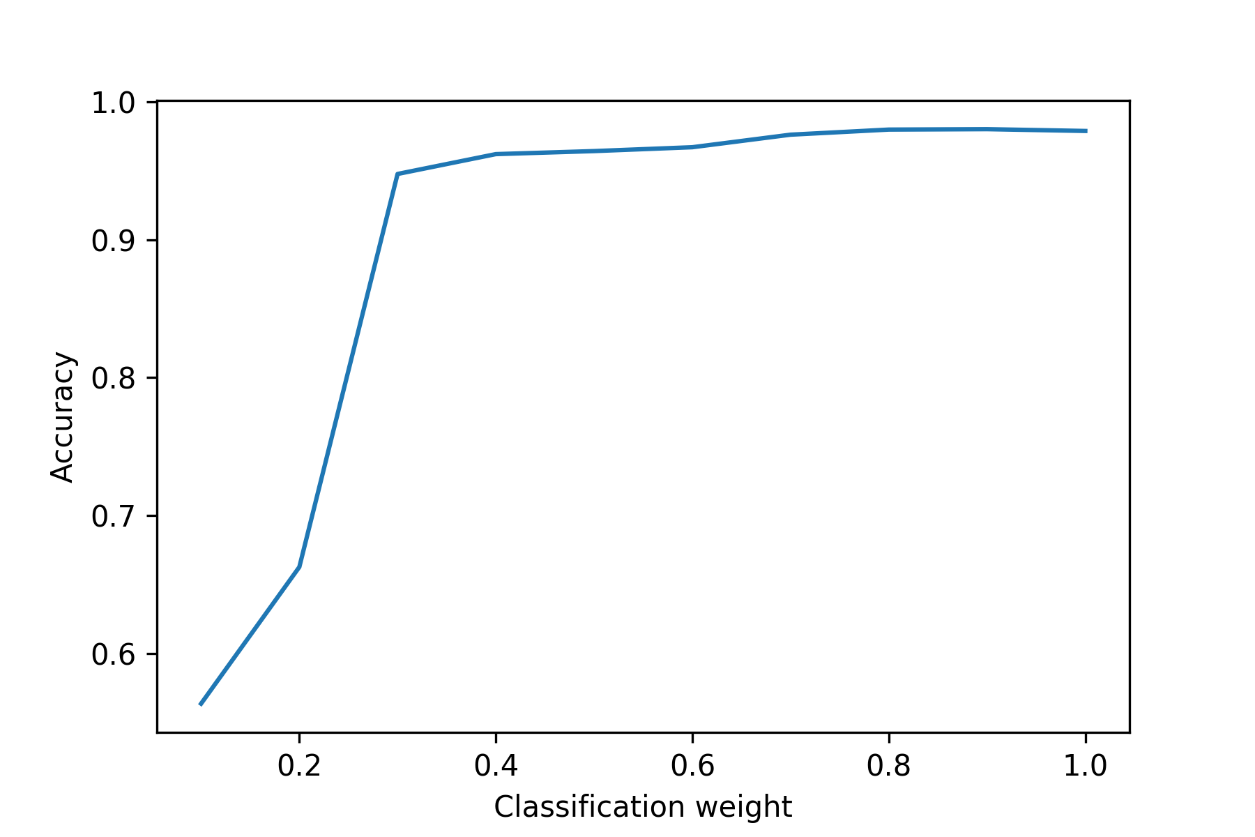
We also checked the accuracy of the ivis classifiers when used to predict the test set labels across the different supervision weights. In general, increasing the supervision weight improved the classifier’s predictive performance on the test set, with maximum performance achieved with a weight of 0.9. At this weight the triplet loss continues to have a small regularizing effect on the results, which may improve the generalizability of the classifier compared to a pure softmax classifier.

Linear-SVM classifier

It’s also possible to utilize different supervised metrics to train the supervised network by adjusting the supervsed_metric parameter. By selecting categorical_hinge it is possible to optimize a linear SVM on the data in conjunction with the triplet loss.

Below is an example of training ivis in supervised mode in tandem with a linear SVM on the Fashion MNIST dataset. Note that the categorical_hinge loss function expects one-hot encoded labels. We can achieve this using the to_categorical function from keras utils.

from tensorflow.keras.datasets import mnist
from tensorflow.keras.utils import to_categorical
from ivis import Ivis
import numpy as np

(X_train, Y_train), (X_test, Y_test) = mnist.load_data()

# Flatten images
X_train = np.reshape(X_train, (len(X_train), 28 * 28)) / 255.
X_test = np.reshape(X_test, (len(X_test), 28 * 28)) / 255.

# One-hot encode labels
Y_train = to_categorical(Y_train)
Y_test = to_categorical(Y_test)

model = Ivis(n_epochs_without_progress=5,
             supervision_metric='categorical_hinge')
model.fit(X_train, Y_train)

embeddings = model.transform(X_test)
y_pred = model.score_samples(X_test)

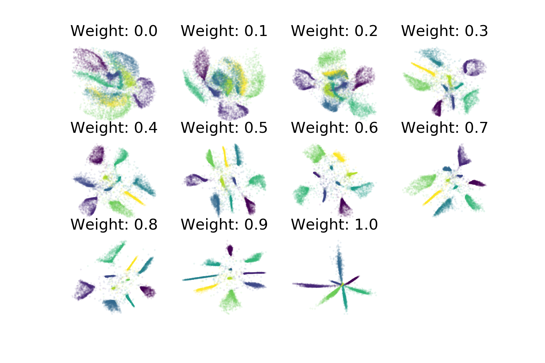
The resulting embeddings show ivis trained with a Linear SVM using the categorical_hinge metric over a variety of supevision_weight values. The maximum achieved accuracy on the test set was 98.02% - once again, a supervision weight of 0.9 led to the highest classification performance.

Multi-label classification

In cases where a single observation is accompanied by multiple response variables, ivis implements support for multi-label classification. Ensuring that y is a multi-dimensional array (N x L), where L is the number of unique labels, multi-label model can be fitted as:

ivis = Ivis(k=30, model='maaten',
            supervision_metric='binary_crossentropy')
ivis.fit(x, y)

Note that the only requirement is that supervision metric is set to binary_crossentropy.

Regression

It is also possible to perform supervised training on continous labels. To do this, a regression metric should be provided to supervision_metric when constructing the Ivis object. Many of these exist in Keras, including mean-absolute-error, mean-squared error, and logcosh.

In the example below, ivis is trained on the boston housing dataset using the mean-absolute-error supervised metric (mae).

from ivis import Ivis
from tensorflow.keras.datasets import boston_housing
import numpy as np

(X_train, Y_train), (X_test, Y_test) = boston_housing.load_data()

supervision_metric = 'mae'
ivis_boston = Ivis(k=15, batch_size=16, supervision_metric=supervision_metric)
ivis_boston.fit(X_train, Y_train)

train_embeddings = ivis_boston.transform(X_train)
y_pred_train = ivis_boston.score_samples(X_train)

test_embeddings = ivis_boston.transform(X_test)
y_pred_test = ivis_boston.score_samples(X_test)

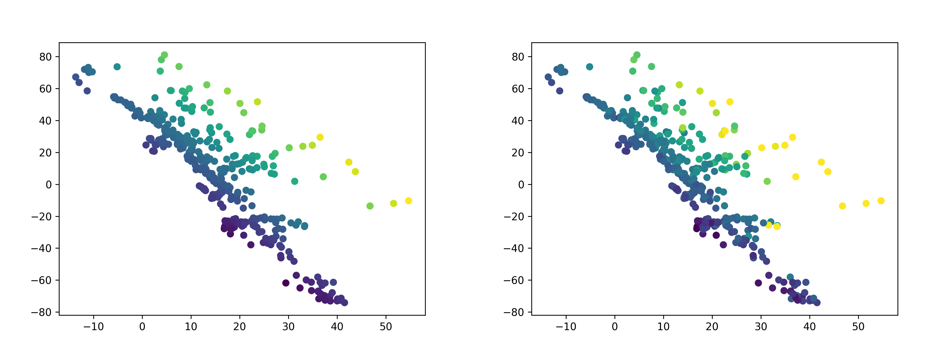
The embeddings on the training set are shown below. On the left are the embeddings are colored by the ground truth label; the right is colored by predicted values. There is a high degree of correlation between the predicted and actual values, with an R-squared value of 0.82.

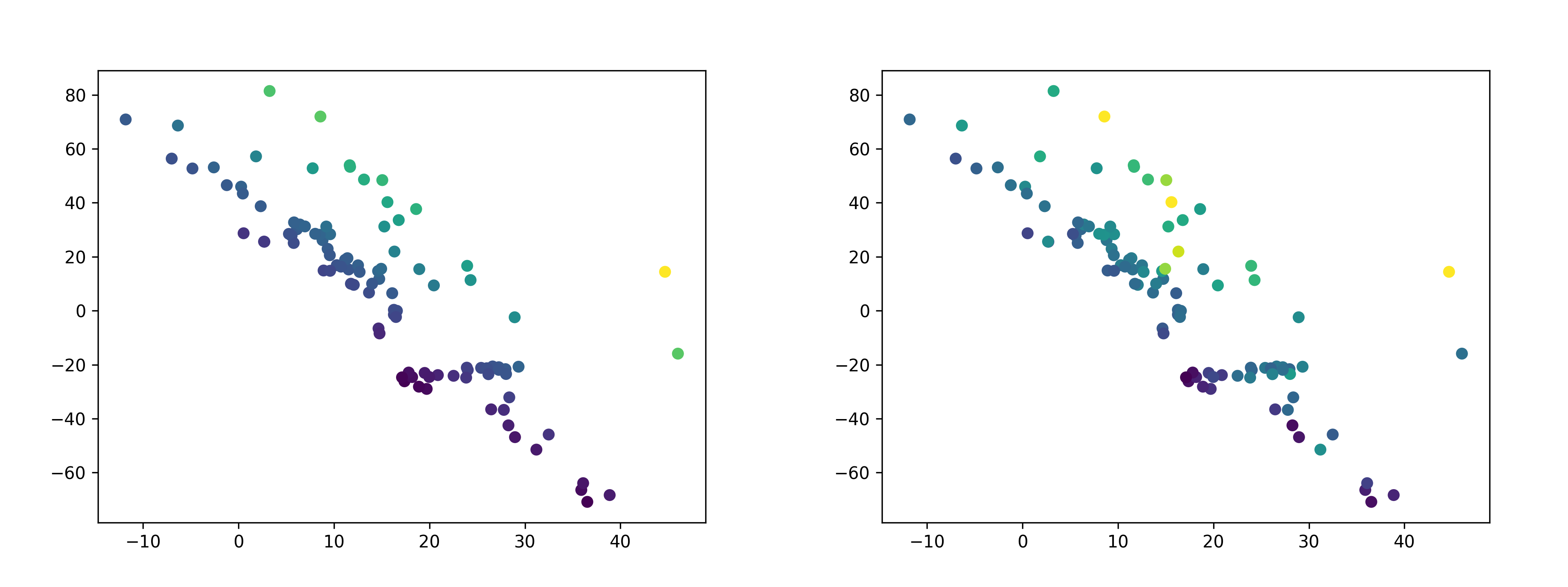
The embeddings on the test set are below. Again, the left is colored by the ground truth label, while the right is colored by predicted values. There is a also a high degree of correlation between the predicted and actual values on the test set, although it is lower than on the training set - the R-squared value is 0.63.

Supervision Weight

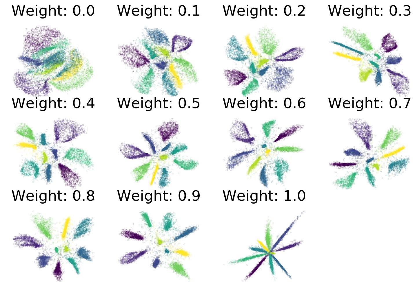
It is possible to control the relative importance ivis places on the labels when training in supervised mode with the supervision_weight parameter. This variable should be a float between 0.0 to 1.0, with higher values resulting in supervision affecting the training process more, and smaller values resulting in it impacting the training less. By default, the parameter is set to 0.5. Increasing it to 0.8 will result in more cleanly separated classes.

weight = 0.8
model = Ivis(n_epochs_without_progress=5,
             supervision_weight=weight)
model.fit(X_train, Y_train)

As an illustration of the impact the supervision_weight has on the resulting embeddings, see the following plot of supervised ivis applied to MNIST with different weight values: